Surface Telerobotics Mission with Astronaut Luca Parmitano

Surface Telerobotics Mission, Session 2, took place on July 26th. Astronaut, Luca Parmitano, controlled our K10 Rover on Earth from the International Space Station. You can see the software we built to control the rover in the below pictures :)

There were lot of media present on the day of the session for coverage, including WIRED, Space.com, etc.

• WIRED: http://www.wired.com/wiredscience/2013/07/nasa-ames-telerobotics/?pid=8511

• Space.com: http://www.space.com/22160-space-station-astronaut-drives-rover.html

• Global News: http://globalnews.ca/news/752773/astronauts-control-rover-from-space/

Surface Telerobotics Mission

So much happened since my last post. I marked my 1 year work-anniversary at NASA on May 28th, 2012. I produced three short films, two of which is related to NASA. One of those videos was shown to the astronaut in the International Space Station, as part of training for our mission: http://youtu.be/Gp_Jj3kzdiM

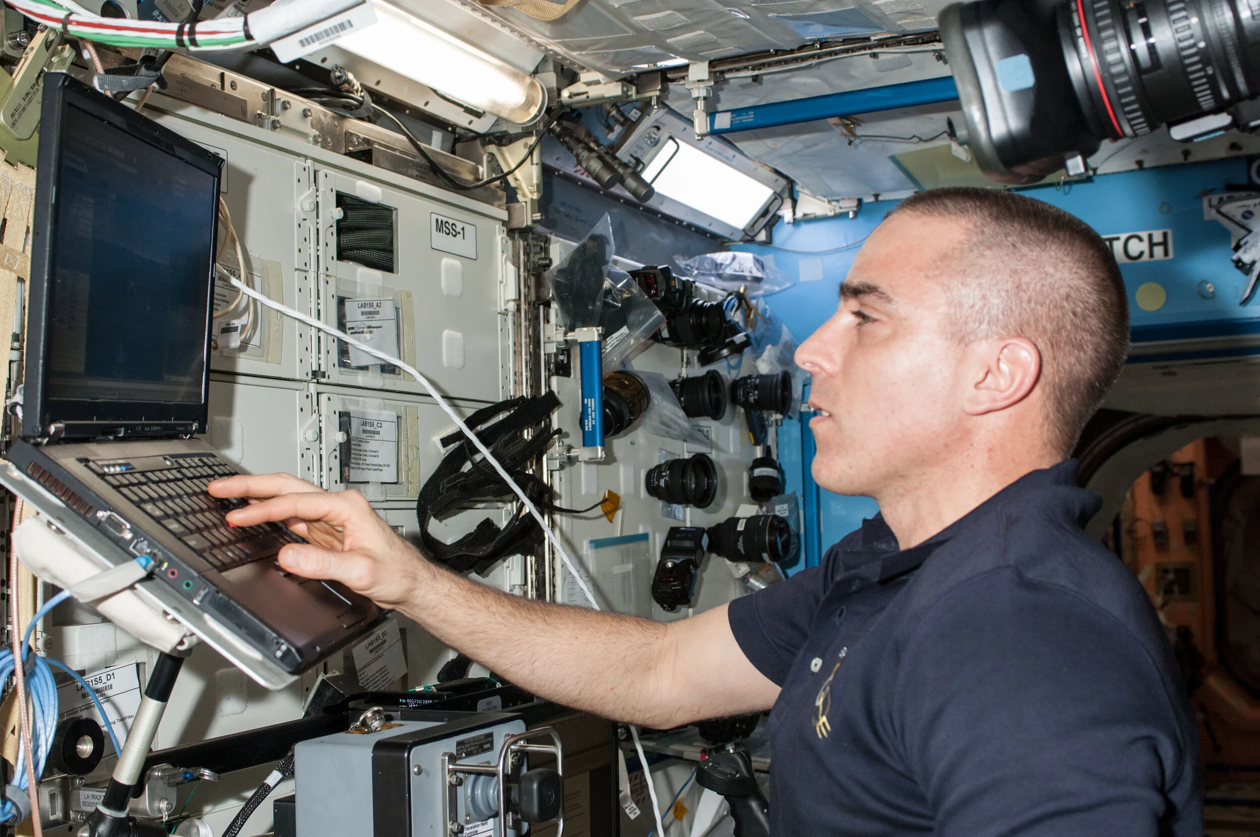
On June 17th 2012, we got to interface with the astronaut on board the ISS as part of our Surface Telerobotics Project. The day started at the crack of down (5am!). There were thankfully no major hiccups and we were able to successfully have the astronaut in space control the K10 rover on Earth! The astronaut who controlled our rover was Chris Cassidy. He's a Navy SEAL, an astronaut, and an engineer from MIT, which officially makes him one of the coolest astronauts ever :) When the session ended, he had only good things to say about the GUI and complimented us on intuitiveness of the controls and the smoothness of the operation. And this of course, made the day for all of us who worked on the project.

Here are high-res pictures sent from the ISS of the astronaut in ISS using our UI to control our rover on the ground:

Image Courtesy of Intelligent Robotics Group at NASA Ames Research Center

Image Courtesy of Intelligent Robotics Group at NASA Ames Research Center

Image Courtesy of Intelligent Robotics Group at NASA Ames Research Center

Factory Method (and other Design Patterns)

While talking about a method inside Verve (3D simulator for robotic control), my teammate said that it was similar to a "Factory". At first, I thought he was making an analogy between an actual factory and the method. But it turned out that he was referring to a pattern called "Factory Method", which was of course outlined in the seminal book "Design Patterns" by Gamma et.al that I conveniently forgot to read after impulsively buying it from Amazon.

Factory Method is a design pattern in object oriented program that allows an instantiation of an object in the subclass instead of the superclass. The superclass would be an interface that outlines the objects that need to be implemented. It is the job of a subclass that implements the interface to instantiate these objects outlined in the interface.

Here's an example. Say you have a Shape super class. Inside the Shape's constructor, it calls a "makeShape" function, which is supposed to instantiate and return a Shape. But the program won't know which shape to make (in another words, "instantiate") because the type of shape is defined in the subclasses. So the job of instantiation is passed to the subclasses of Shape super class, such as Circle. Circle Subclass would implement the "makeShape" method that instantiates the shape and returns it.

There is another pattern that is similar to Factory Method but does not instantiate each time but rather passes back the same object that was instantiated once for that class. It's called a "Singleton".

Geometry Clipmaps

I am currently reading a paper called "Geometry Ciipmaps: Terrain Rendering Using Nested Grids" by Frank Losasso and Hughes Hoppe, for my next project in IRG for terrain-rendering related project.

What is a Geometry Clipmap: 

It caches the terrain in a set of nested regular grids (which are filtered version of the terrain at power of two resolutions) centered about the viewer and it's incrementally updated with new data as the viewer moves.

What is the difference between Mipmaps / Texture Clipmaps / Geometry Clipmaps ? 

A mipmap is a pyramid of images of the same scene. The set of images goes from fine to coarse, where the highest mipmap level consists of just one pixel. Mipmap level rendered at a pixel is a function of screen space parametric derivatives, which depend on view parameters and not on the content of the image.

A texture clipmap caches a view dependent subset of a mipmap pyramid.  The visible subset of the lower mip levels is limited by the resolution of the display. So it's not necessary to keep the entire texture in memory. So you "clip" the mipmap to only the region needed to render the scene. Texture clipmaps compute LOD (level of detail) per-pixel based on screen space projected geometry.

With terrains, geometry for screen space does not exist until the level of detail is selected. But texture clipmaps compute LOD per-pixel based on existing geometry. See the problem?

So geometry clipmaps selects the LOD in world space based on viewer distance. It does this by using set of rectangular regions about the view point and uses transition regions to blend between LOD levels.

Refinement Hierarchy

Geometry clipmap's refinement hierarchy is based on viewer centric grids but ignores local surface geometry.

Overview of Geometry Clipmap

Consists of m levels of terrain pyramid. Each level contains n x n array of vertices, stored as vertex buffer in video memory. Each vertex contains (x,y,z,z_c) coordinates, where z_c indicates height value at (x,y) in the next coarser level (for transition morphing).

Texture

Each clipmap level contains associated texture image(s), which are stored as 8-bit per channel normal map for surface shading (more efficient than storing per-vertex normals. The normal map is computed from the geometry whenever the clipmap is updated.

Per-frame Algorithm

• determine the desired active regions (extent we wish to render)

• update the geometry clipmap

• crop the active regions to the clip regions (world extent of nxn grid of data stored at that level), and render.

Computing Desired Active Regions

Approximate screen-space triangle size s in pixels is given by

eq1

W is the window size

phi is the filed of view

If W = 640 pixels, phi = 90 degrees, we obtain good results with clipmap size n=255.

Normal maps are stored at twice the resolution, which ives 1.5 pixels per texture sample.

Geometry Clipmap Update

Instead of copying over the old data when shifting a level, we fill the newly exposed L-shaped region (since the texture look up wraps around using mod operations on x and y). The new data comes from either decompressing the terrain (for coarser levels), or synthesizing (for finer levels). The finer level texture is synthesized from the coarser one using interpolatory subdivision scheme.

Constraints on the clipmap regions

• clip regions are nested fro coarse-to-fine geometry prediction. Prediction requires maintaining one grid unit on all sides.

• rendered data (active region) is subset of data present in clipmap (clip region).

• perimeter of active region must lie on even vertices for watertight boundary with coarser level.

• render region (active region) must be at least two grid units wide to allow a continuous transition between levels).

Rendering the Geometry Clipmap

//crop the active regions

for each level l = 1:m in coarse-to-fine order:

  Crop active_region(l) to clip_region(l)

  Crop active_region(l) to active_region(l-1)

//Render all levels

for each level l=1:m in fine-to-coarse order:

  Render_region(l) = active_region(l) - active_region(l+1)

  Render render_region(l)

Transition Regions for Visual Continuity

In order to render regions at different levels of detail, the geometry near the boundary is morphed for each render region s.t. it transitions to geom of coarser level.

Morphed elevation (z'):

eq2

where blend parameter alpha is computed as alpha = max(alpha_x, alpha_y).

eq3

v'_x denotes continuous coordinates of the viewpoint in the grid of clip region.

x_min and x_max are the integer extents of the active_region(l).

Texture Mapping

Each clipmap level stores texture images for use in rasterization (i.e. a normal map). Mipmapping is disabled but LOD is performed on the texture using the same spatial transition regions applied to the geometry. So texture LOD is based on viewer distance rather than on screen-space derivatives (which is how hardware mipmapping works).

View-Frustrum Culling

pic2

For each level of clipmap, maintain z_min, z_max bounds for the local terrain. Each render region is partitioned into four rectangular regions (see Figure 6). Each rectangular region is extruded by zmin and zmax (the terrain bounds) to form a axis-aligned bounding box. The bounding boxes are intersected with the four-sided viewing frustum and the resulting convex set is projected onto an XY plane. The axis aligned rectangle bounding this set is used to crop the given rectangular region.

Terrain Compression

Create a terrain pyramid by downsampling from fine terrain to coarse terrain using a linear filter. Then reconstruct the levels in coarse-to-fine order using interpolatory subdivision from next coarser level  + residual.

Terrain Synthesis

Fractal noise displacement is done by adding uncorrelated Gaussian noise to the upsampled coarser terrain. The Gaussian noise values are precomputed and stored in a look up table for efficiency.

Here are some good references:

A good follow up paper: http://research.microsoft.com/en-us/um/people/hoppe/gpugcm.pdf

Awesome website on terrain rendering: www.vterrain.org

Destination Innovations features IRG!

Cool video illustrating different Human-Robot Interaction Projects currently in development at Intelligent Robotics Group (where I work :D ).

Brushing up on Probabilities, Localization, and Gaussian

Gaussian: It is a bell curve characterized by mean and variance. It's is unimodal and symmetric. The area under the Gaussian adds up to 1.

Variance: measure of uncertainty. Large covariance = more spread = more uncertain.

Bayes Rule

Localization:

Involves "move" (motion) step and "sense" (measurement) step.

Motion (move) : First the robot moves. We use convolution to get the probability that robot moved to the current grid location. We use Bayes Rule (given previous location, find probability of being in this current grid location).

Measurement (sense) : Then robot senses the environment. We use products to get the probability that the sensor measurement is correct. Measurement applies theorem of total probability (sum of:  probability that sensor measurement is correct given it's a hit, prob that sensor is correct given it's a miss).

*Side note: for grid based localization method (histogram method), the memory increases exponentially with number of state variables (x,y,z, theta,row, pitch, yaw, etc) 

Intel SDK for OpenCL Applications Webinar Series 2012

Intel hosted a webinar on running OpenCL on Intel Core processor. The webinar I attended this morning (9am, July 11th), is first part of the three-part webinars on this topic. It was well organized and educational and I think the next seminar will be even more useful (since it deals with programming using OpenCL. I took notes during the webinar to get you up to speed in case you want to attend the next two seminars.

* July 18-Writing Efficient Code for OpenCL Applications<http://link.software-dispatch.intel.com/u.d?V4GtisPHZ8Stq7_bNj1hJ=3231> * July 25-Creating and Optimizing OpenCL Applications<http://link.software-dispatch.intel.com/u.d?K4GtisPHZ8Stq7_bNj1hS=3241> 

OpenCL: Allows us to swap out loops with kernels for parallel processing.Introduction: Intel’s 3rd Generation Core Processor.

• Inter-operability between CPUs and HD Graphics.
• Device 1: maps to four cores of intel processor (CPUs)
• Device 2: Intel HD Graphics.
• Allows access to all compute units available within system (unified compute model - CPU and HD Graphics)
• Good for multiple socket cpu - if you want to divide the openCL code with underlying memory architecture.
• Supported on Window7 and Linux.

General Electric’s use of OpenCL

• GE uses OpenCL for image reconstruction for medical imaging (O(n^3) - O(n^4))
• Need unified programming model for CPUs and GPUs
• OpenCL is most flexible (across all CPU and GPUs) - good candidate for unified programming language.
• Functional Portability: take OpenCL application and run it on multiple hardware platforms and expect it to produce correct results.
• Performance Portability: functional Portability + Deliver performance close to entitlement performance (10-20%)
• Partial Portability: functional Portability + only host code tuning is required.
• Benefits of OpenCL:
  • C like language - low learning curve
  • easy abstraction of host code (developers focus on kernel only)
  • easy platform abstraction (don’t need to decide platform right away.)
  • development resource versatility (suitable for mult. platforms)
• Uses combination of buffers (image buffers and their customized ones). Image buffers allow them to use unique part of GPU.
• Awesome chart that compares various programming models:

Intel OpenCL SDK: interoperable with Intel Media SDK with no copy overhead on Intel HD Graphics.Intel Media SDK: hardware accelerated video encode/decode and predefined set of pre-processing filtersThank you UC Berkeley Visual Computing Center for letting me know about this webinar series!

AI Course on Udacity

I've been taking an artificial intelligence course on Udacity (http://www.udacity.com/courses), an online course taught by Sebastian Thrun. The course is called "Programming a Robotic Car". One of my co-workers pointed out that the course covers exactly what I need to learn - probabilities, Kalman Filter, Particle Filter, and SLAM. I will be blogging about my progress with the course and the insights I picked up from it.

Unlike OpenCourseWare from MIT and other webcasts offered, Udacity is much more interactive. I didn't find myself bored or distracted (though I'm taking a break right now to write this blog) because it has short quizzes (they are easy and very short) to recap the concepts covered in the video. The videos also focus on insight and doesn't dwell on the mathematical formulation of the problem unless it's absolutely necessary. And as a visual learner, I find Sebastian Thrun's drawings very helpful in understanding the concept.

I wish every web classes offered online were as good as these. I hope you find them useful.

Understanding FastSLAM

The SLAM I’m talking about has nothing to do with poetry or basketball. I’m “investigating” (read “learning on the fly") the SLAM algorithm (Simultaneous Localization and Mapping). One of my co-workers forwarded me two papers that I should read (http://tinyurl.com/6vfvuxg), both of which are co-authored by Sebastian Thrun of Google X (clearly I am very excited to point this out). I think it’s pretty awesome that reading research papers is part of my job.

To understand FastSLAM (version of SLAM in the papers), I needed to understand particle filter and Kalman Filter. Here are one sentence summaries based on wikipedia articles:

particle filter: Uses differently weighted samples of distribution to determine probability of an ‘event happening’ (some hidden parameter) at a specific time given all observations up to that time.

*note to self: similar to importance sampling: particle filter is more flexible for dynamic models that are non-linear.

Kalman Filter: Takes in a noisy input and using various  measurements (from sensor, ctrl input, things known from physics), recursively updates the estimates (they call it system’s state) to be more accurate. example: A truck has a GPS that estimates the position within few meters.  Estimate is noisy but we can take into account the speed and direction over time (via wheel revolution and angle of steering wheel) to update the estimated position to be more accurate.

*note to self: Kalman Filter assumes linearity in dynamics and in noise.

In terms of flexibility, it can be described this way (from least flexible to most):

Kalman Filter < Exteneded

Kalman Filter < Particle Filter

FastSLAM is a Bayesian formulation. It essentially boils down to this:

The particle filter is used to estimate the path of the robot (it’s given by the posterior probability p(s_t | z_t, u_t, n_t)). First, construct a temporary set of particles from robot’s previous position and the control input. Then sample from this set with probability of importance factor (particle’s weight). Finding weight of each particle is quite involved. I’ll let you refer to the actual papers for the derivation.

After we have path estimates, we can solve for landmark location estimates (the right side of the equation). Through series of equalities, authors arrive at:

FastSLAM updates the above equation using the Kalman Filter.

The main advantages of FastSLAM are that it runs at O(M log K) instead of O(MK), where M is number of particles, K is number of landmarks. I've had trouble understanding this part but here it goes: each particle contains the estimates of K landmarks (and each estimate is a Gaussian). Resampling particles requires copying the data inside the particle (K Gaussians if we have K landmarks). Instead of copying over all K landmark location estimates, FastSLAM does a partial copy for only Gaussians that need to be updated. Also the conditional independence between landmark location and robot location allows for easy setup for parallel computing.

Stay tuned for breakdown of FastSLAM2.0 ...